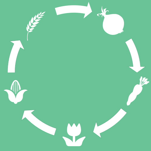
Dutch people are pretty level-headed. You don’t hear Dutch people say that we are the greatest country on earth, or that we have the best food. But the Dutch sometimes forget to be proud of what they have accomplished. After years of battling the sea, specifically the ‘Zuiderzee’, we had enough and turned this sea into a lake. But maybe the biggest accomplishment of all is that we have created our own land: Flevoland. Since 1950 we have built an entire extra province. After having suffered many food shortages during war periods, Flevoland was constructed to secure food supply. Flevoland turned out to host the most fertile soil of the Netherlands. These days, about four times as much crops are grown per square meter in Flevoland compared to the rest of the Netherlands. A lot of these super-fertile fields are owned by the government, and leased to farmers. In order to ensure that the quality of the soil remains high and to avoid diseases in the ground, a crop rotation plan needs to be followed, see Figure 1. Crop rotation plans are therefore imposed on the farmers by the government.

*Figure 1: A schematic representation of a crop rotation plan. Planting different crops each year is beneficial for the fertility of the soil.*

To ensure that the crop rotation plans are followed, the fields owned by the government are visually inspected by car. That means that someone has to drive to all the fields, measure which crop grows where, and then checks if it is in line with the crop rotation plan. This currently takes up a lot of time. This is where we come in.

So how can we speed up this process? One way is to inspect the fields with drones. This way more fields can be inspected in one view. However, drones can be expensive and ground operations still need to be setup for controlling the drone. We from Geronimo.AI have taken it a step further. We can detect all the crops in Flevoland in one go, and we do this from space!

We have developed a pipeline that uses machine learning and satellite data to create a crop map of Flevoland, showing objectively which crops are grown on which fields. In the following sections, I will explain the steps that we take in order to go from satellite imagery to a crop map of Flevoland.

The input data

Detecting crops from satellite imagery can be challenging. First of all, unless spending a lot of dollars, satellite imagery in general has a pretty low resolution. So using visual features for detecting crops would be very difficult. However, there might be different methods to extract a characteristic signal from imagery. By including the time dimension into our signal, the characteristic features of the development of a crop can be extracted. We do this by extracting time series of the Normalised Difference Vegetation Index (NDVI) of each parcel. The NDVI is a measure of how much light a plant absorbs. NDVI is based on the following equation:

NDVI =(NIR – VIS)/(NIR + VIS)

where NIR = Near Infrared light, and VIS is Visible red light.

By building a time-series of the NDVI we can see the different phenological stages a plant is in. These signals are characteristic for each crop, as can be seen in Figure 2, and are also referred to as ‘growth curves’.

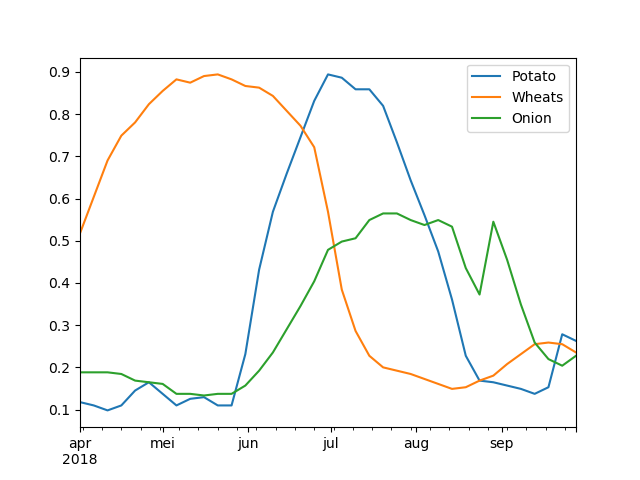
*Figure 2: Normalised Difference Vegetation Index (NDVI) of potato, wheats, and onion plotted against the time of the year. There is a clear distinction between the individual NDVI curves.*

These signals can be fed to a machine learning model, if we have a labelled dataset that couples each curve to a crop. The trained machine learning model would then be able to detect a crop, given an NDVI curve.

But how do we generate these NDVI curves?

The NDVI curves are a product of satellite imagery and we have chosen to use the Sentinel 2 satellites from the Copernicus programme as our main multispectral input data source. The Copernicus program is a satellite programme by ESA with the goal of freely giving access to different earth observation satellites. The first satellite was launched in 2014, and a number of satellites for different purposes are still to be launched. Sentinel 2 has a resolution of 10m per pixel, and has a revisit time of about 3 days for each part of the earth.

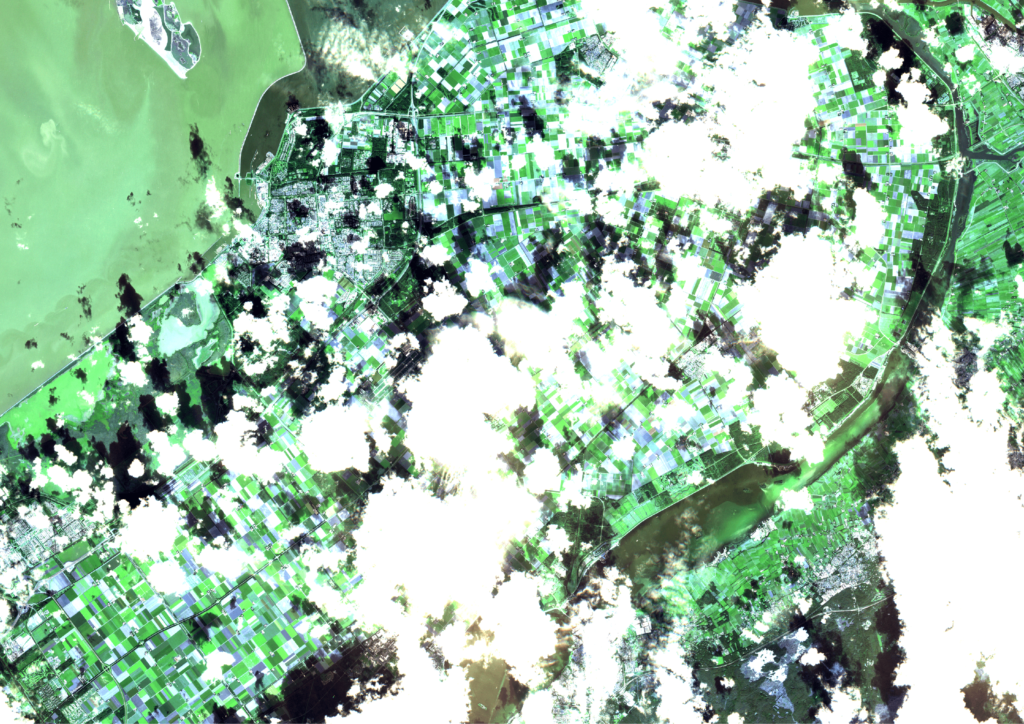
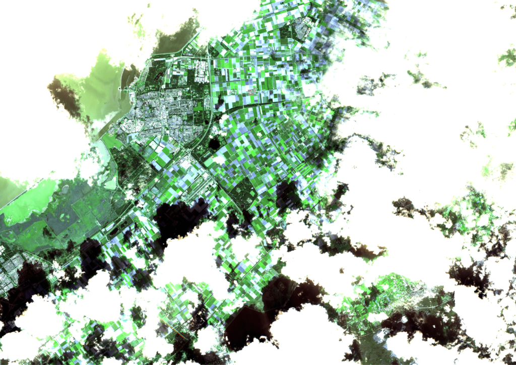
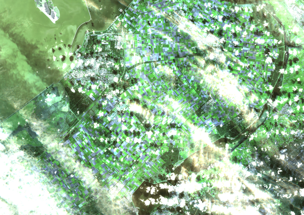
However, as the weather in the Netherlands is quite suboptimal, a lot of recordings are useless, because they are fully covered by clouds. Only recordings that have a certain cloud cover percentage are processed. Even then, a lot of the images are still partially cloudy, as can be seen in the following three consecutive recordings of Flevoland in September. These clouds and cloud shadows still need to be filtered out of the image, such that a masked image with valid and invalid pixels remains.

Figure 3: Cloudy recordings of Flevoland. Clouds pose a problem because they hinder the detection of NDVI values. Therefore clouds need to be detected and masked, such that they do not pollute the NDVI signals.

Expanding the input data with radar images

An early experiment showed good results on predicting crops given an NDVI curve. This experiment was performed on a training and test dataset from 2018. Afterwards, we found out that 2018 was a really good year with regard to cloud cover in the Netherlands. Results for 2019 were a lot worse, because accurate NDVI curves proved difficult to construct under very cloudy conditions. The data input pipeline was therefore extended with radar imagery from the Sentinel 1 constellation. Because radar is an active sensor, it can still get a signal when it is cloudy. However, radar does not measure NDVI but the backscatter of the signal it is transmitting. Sentinel 1 polarises the radar signal in two modes, VV and VH, see Figure 4. Images can be made from the backscatter coefficients of the VV and VH imagery, comparable to the NDVI image that is created from the Sentinel 2 bands. The VV and VH signals contain information about the texture and roughness of a surface, hence it can be characteristic for different crops.

*Figure 4: An example of a recording from the Sentinel 1 satellite. Here the VH polarisation is shown.*

Now that we have our data sources in order, we can start with the fun part, the machine learning part!!

Learning to detect crops

So we have processed our input data, now we can simply train a model and we are done right? Well not really, there is still one important piece missing, a labelled dataset. We now have defined our steps on how to process the satellite imagery to NDVI curves. However, we still need to build a dataset of NDVI curves coupled with the correct crop. Luckily the Dutch government has a lot of open datasets about the use of agricultural land in the Netherlands. The Basisregistratie GewasPercelen (BRP) is the main dataset we can use for acquiring a labelled dataset. The BRP contains the geographical boundaries of each individual parcel in the Netherlands, coupled with the crop that is grown on it. It contains over 780,000 individual agricultural parcels of the Netherlands, most of them being grasslands though.

*Figure 5: Individual parcels from the Basisregistratie GewasPercelen (BRP).*

But if there already is a dataset of all the crops in Flevoland, why are we then trying to predict the crops with machine learning? Well the answer is that we want to have a tool that is able to detect the ground truth. And since the BRP is a result of a documentation of each owner of every parcel, we cannot be sure that it is always true. In fact, frauding farmers are probably also misleading the BRP. If we are able to build a tool that gives insight in which crops grow where, we are able to compare it with the BRP and catch anomalies. In addition we are able to check if crop rotation plans are followed by not only looking at the BRP, but by using the ground truth!

So how exactly do we use the BRP to generate a labelled dataset of NDVI curves? We could make a dataset of labelled NDVI time-series for each pixel, by looking in which crop parcel the pixel is located. However, we opted for a different approach by simply taking the median NDVI pixel value of each crop parcel, and constructing time-series of these values. This way the dataset is much more compact, while still catching most of the variation in the data.

Because the BRP has over 100 crop categories, we combine certain crops that are very much like eachother, and only use the most occuring crops to make life a bit easier for the machine learning model. After combining crops and only selecting the 11 most occuring crops, we still have about 90% of the original dataset. Now we can start training a machine learning model to predict the crop category, given an NDVI curve.

Let’s start training!

Now that we have all the input and target data ready, we can start to train a machine learning model. Because of the medium to high input dimensionality we opted for using a deep learning approach. For each month, a model optimisation was performed to select the best pre-processing parameters. Because the dataset was made relatively small, training converged in just a few minutes on a local Nvidia GPU.

Analysing the results

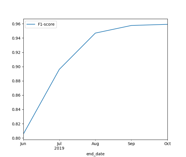
We were very curious to see how training a model and making a prediction for the current year would improve as time progresses. Figure 6 below shows the progression of the F1-score with the end date that the model is trained on. What is interesting to see is that there is almost no difference between making a prediction in September and making a prediction in October. So most of the crops do not gain a lot of characteristic signal after September, having completed most of their growth curve. In addition, a lot of the crops are already harvested during that time of the year. However, Figure 6 also shows that we still have a decent F1-score when making a prediction in June, which is quite a nice result!

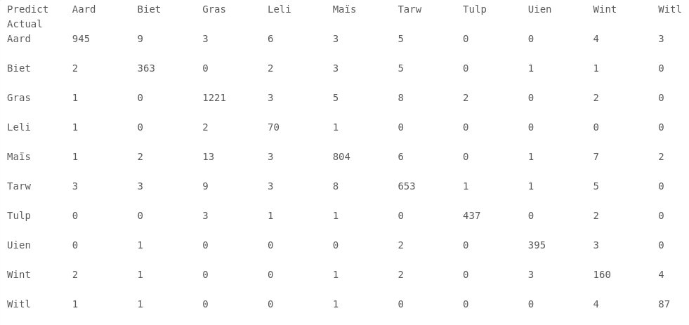
Figure 6: Evolution of F1-scores as the year progresses. It can be seen that a model that is trained on a longer satellite signal performs better. However, training a model on October does not bring that much extra performance with respect to a model trained on September.

What is very interesting to see is the confusion matrix for the model trained on the time-series up to October, which is shown below. The names of the crops are the Dutch names abbreviated to 4 letters. From this confusion matrix we can see that most crops have a high classification accuracy. We can also see that grasslands are sometimes confused with corn (maïs) or other crops. An interesting question is whether this is an error in the model, or an error in the BRP administration which generates the ground truth for the validation data.

*Figure 7: Confusion matrix of the model that was trained on time-series up to October.*

Building a crop map of flevoland.

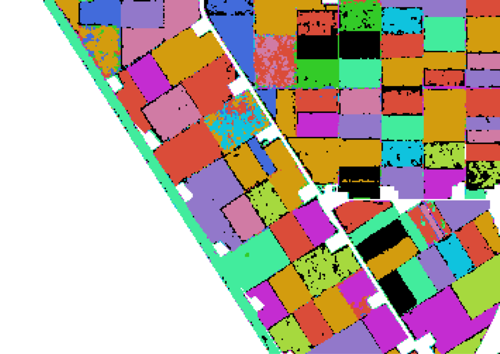
So far we have shown results in numbers. Not very exciting right. One cool idea is to apply the trained algorithm on every pixel of the imagery, thereby creating a crop map. Well, we have done exactly this. The result for a small portion of Flevoland can be seen below in this fancy slider.

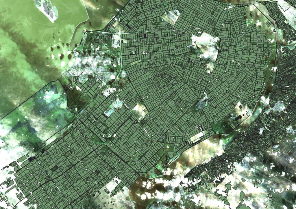
Cool right? We can see that the algorithm performs quite accurate as we can easily detect the individual parcels with crops in the images. The cool thing about using satellite data is the scalability of the solution: we can now build an entire crop map of Flevoland and Noord-Holland:

Detecting interesting features with the crop map.

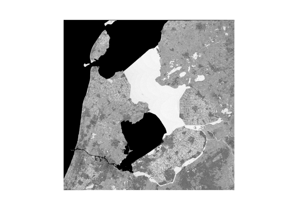
Now that we have our crop map, we can start playing around with it. One of the most interesting things is to check how well the crop map matches with the BRP that holds all the crops as submitted by the farmers. In the following image, the black pixels denote a deviation from the prediction with the BRP. We can see a few suspicious parcels that are fully black. However it is difficult to judge whether this is a model error or whether the BRP is faulty. The only way to find out would be to do a field inspection.