Humans are really good at understanding and interpreting language. Think about it, once you read a sentence you can interpret its underlying sentiment without any effort. We can even understand sarcastic comments from written language, which basically is the easiest thing in the whole world, like duh. Extracting subjective information from text, however, is way harder for a computer. This task is often referred to as sentiment analysis.
This blog is the first of three rather technical blogs and will introduce you to the Naive Bayes classification algorithm. We will use the algorithm to classify movie reviews as either positive or negative, for which we will use the famous IMDB dataset of 25k positive and negative reviews. This blog will mainly focus on the pre-processing of data; splitting up sentences in words, how to remove redundant information and how to focus on statistically relevant words. The second blog will investigate the design choices that can be made with feature selection. Finally, the third blog will explore the performance of the algorithm on unbalanced datasets.
[latexpage] I want you to think about sentiment analysis a bit more. How do you define a classifier for this task? We have several classes or sentiments $C$, in our case positive and negative and we have a review $R$. Now we are interested in what class or sentiment $c \in C$ this review $R$ falls. Warning: maths ahead!
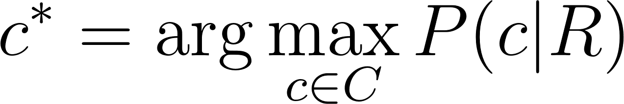
More formally, we are interested in a function that returns the class with the highest probability given the review:
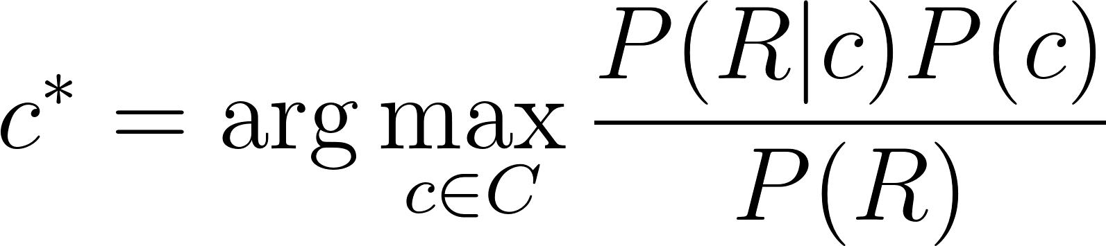
Now using bayes’ theorem we can rewrite this equation as:
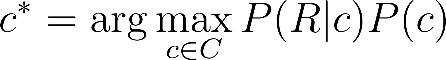
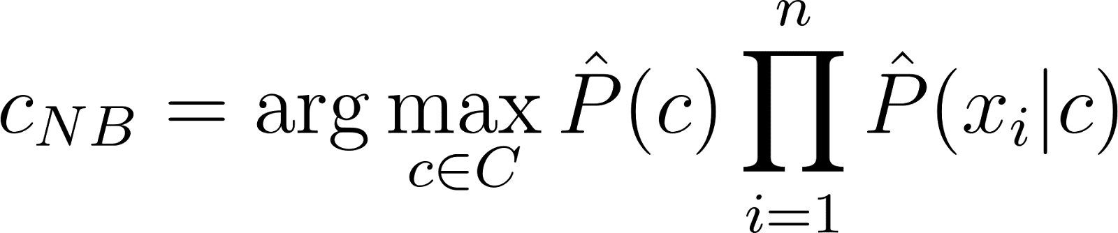
[latexpage] Since we maximize over $c$ and $P(R)$ is not dependent on $c$, so we can leave that out of the argmax equation. An intuitive way to think about this is that for any class in all classes the probability on the review $P(R)$ is exactly the same, regardless the class and therefore it does not influence the maximum. Hence, we can simplify as:
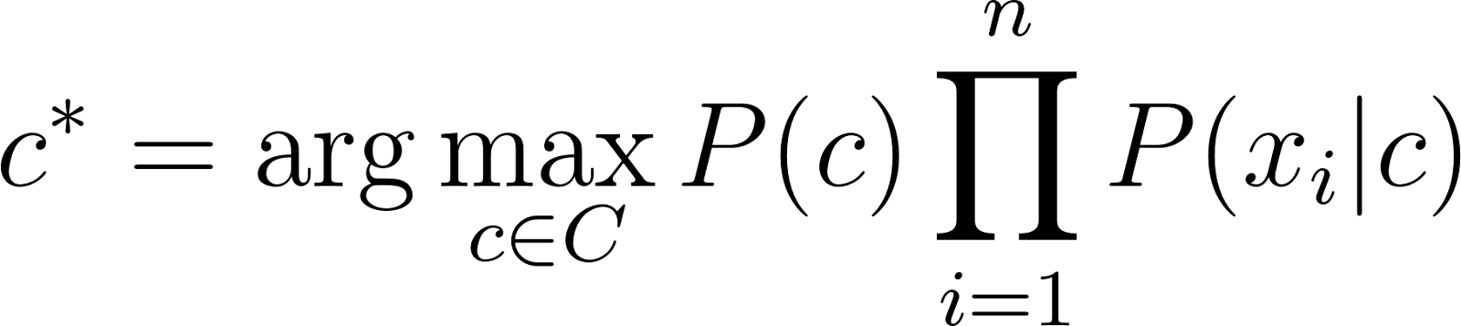
[latexpage] Suppose we are a bit naive and present a review as a bunch of features $x_1, x_2, \dots , x_n$, which are the words in the text. By doing so, we implicitly assume that the class to which our review $R$ or list of features $x_1, x_2, \dots , x_n$ belongs, does not depend on the order of the words. A review is now a list of features $R = [x_1, x_2, \dots , x_n] = [x_2, x_n, \dots , x_1]$ or any order for that sake. Plugging this into the equation results in:

[latexpage] In fact, we now have a classifier. Given a set of reviews $\mathcal{R}$ we can simply count the occurences of the classes to approximate $P(c)$. The issue is however with the term $P(x_1, x_2, \dots , x_n \vert c)$. Using the probability chain rule, we can rewrite this expression. Given a review (“Best movie ever!”) we could rewrite this term as:

[latexpage] Here each probability can be extracted from the data. Here, for example $P(x_3 \vert x_2, x_2, c)$ is interpret as the chance on “ever” given the features “best” and “movie” and class $c$. However, these probabilities are very specific and as the reviews get larger, these probabilities get more and more specific. For example, take the following probability $P(x_{100} \vert x_{99},… x_{1}, c)$. The chance on the last word of a review, given all the other words in the review, would be a very unique probability. We can be pretty sure that we do not encounter this exact probability in another set of reviews, since it is unlikely that a review has exactly the same content of another review. This results in the need of a very large dataset to get an estimate of the probabilities, making this approach infeasible. We therefore need to look at another way of classifying a review given the words in that review. Would there be a way where we could just look at the occurrence of individual words?
There is. What if we assume that the words are conditionally independent. Conditional independence in this case can be interpreted as follows. If we consider the words in all the reviews together they are dependent of each other. Now however, if we take a look at the words from specific class, we assume these words occur independently within each class. By making this assumption we can therefore rewrite our chance as:

We now only need the chance of a word in occurring in a class, which is appearing way more often. Plugging this into the main equation results in:
[latexpage] Now the most common approach to estimate our probabilities is using the frequencies in the data. So for $P(c)$ we can count the number of documents in class $c$ and divide them by the total number of documents and for any word probability in a class $P(x_i \vert c)$ we can count how often that word $x_i$ occurs in class $c$ and divide it by the total number of words in class $c$, resulting in:
Well, there you have it! By making two naive assumptions 1) that the word order does not matter and 2) that the words are conditionally independent, we now have derived the Naive Bayes classifier. Although trivial, the Naive Bayes is known to be a robust and fast classifier for binary text classification.
[latexpage] Think a second about the term $\prod_{i=1}^n \hat{P}(x_i \vert c)$ in the classifier equation. What is the big shortcoming of this term? You’ve guessed it! If there are words present in the test set, which are not present in the train set or if words are not present in each class $c \in C$, its probability approximation is 0, which cancels out all other approximations. This can destroy valuable information, which is unwanted. Currently, we approximate the probability for $x_j$ with $j \in [1, n]$ as:
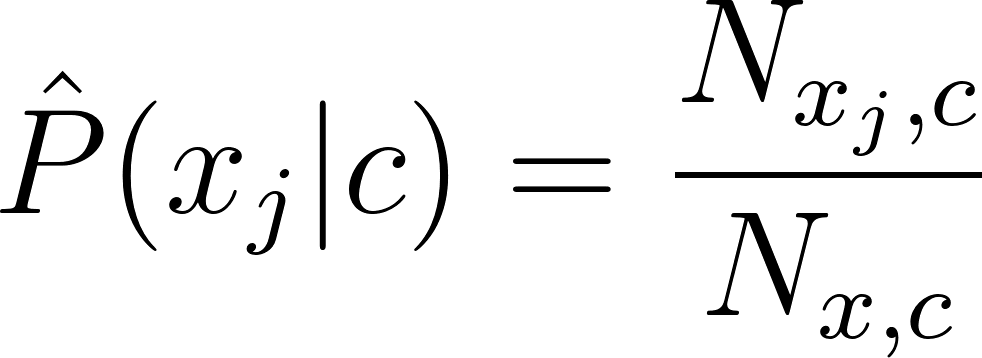
[latexpage] Here $N_{x_j, c}$ is the number of times the word $x_j$ occurs in class $c$ and $N_{x, c}$ is the total number of words in class $c$.
[latexpage] We can prevent the zero terms by smoothing this expression. Smoothing is done by adding $\alpha$ to each word occurrence $x_j$ resulting in the following expression:
[latexpage] where $n$ is the total number of unique words.
[latexpage] Parameter $\alpha$ is a tuning parameter of the algorithm, which is usually fixed at $\alpha = 1$. If that is the case, we call it laplace smoothing
Naive Bayes in practice
Congratulations! You have made it through the mathematical derivation of Naive Bayes. From here on we will discuss common ways of pre-processing data when it comes to the usage of Naive Bayes for text classification. We will also investigate their impact on accuracy and number of features by running a bunch of experiments.
Tokenization
The first design choice we have to make is how to split the reviews into words. This process is often referred to as tokenization, where the words are called tokens. In similar fashion, a tokenizer is a function that takes a full sentence as input and returns a set of tokens as output. There are many tokenizers out there, but we will consider two.
We will compare the build-in tokenizer in sk-learn with the more advanced tokenizer provided by Spacy. Sk-learn and Spacy are famous python libraries often used in the field of machine learning and NLP (feel free to give it a go on Google to verify 🙂 ). Spacy provides more advanced language models, whereas sk-learn provides easy-to-use implementations of most common machine learning techniques.
Stopword removal
Common practice is to remove stopwords for the set of words that are used as features, since they do not contribute to a specific class, therefore overshadowing words that actually carry more sentimental information. You can image that words such as ‘since’, ‘all’ and ‘however’ occur roughly as often in negative as in positive reviews.
TF-IDF
There is interest in removing words with a higher document frequency with the idea that these overrule more uncommon words. One way of reaching this is stopword removal. However, this is not very situation specific and you can imagine that each problem has their own set of words that occur very often. In our case you can think of words as “movie” which will occur in both positive (“Best movie ever!”) and negative (“This movie is terrible”) reviews, but does not contain much sentiment.
[latexpage] One way to “downsample” more frequent samples and give more value to less frequent words is the to take each term frequency (TF) and multiply it with its inverse document frequency (IDF), which is called TF-IDF. In that case, the approximation of the probability of feature $x_j$ is given as:
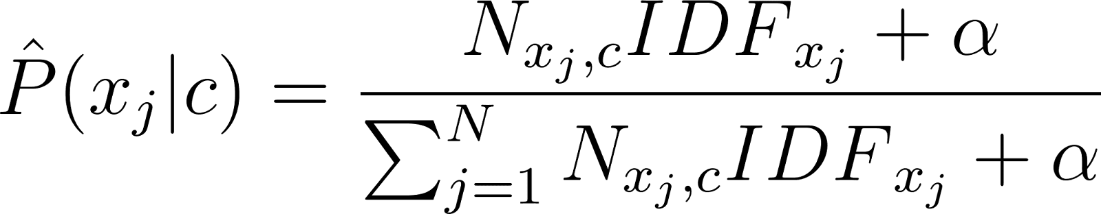
[latexpage] Here $N_{x_j, c}$, $N_{x, c}$ and $n$ are as previously defined. There are several formulas for $IDF_j$ available, but in this blog we will use the one used in sk-learn calculated as:
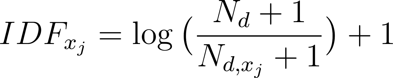
[latexpage] Here $N_{d,x_j}$ is the number of documents that contain the term $x_j$. Note that this is independent of class $c$. Furthermore, $N_d$ is the total number of documents in the dataset, which is not the same as $\sum_{j=1}^N N_{d, x_j}$. The +1 term in the numerator and denominator within the log prevent zero division, where as the +1 on the outside prevents an approximation of zero.
The presented formulas are the implementations used in sk-learn, where they use an extra step to normalize the TF-IDF values with respect to the vector of the whole document. For a detailed explanation, please see the user guide of sk-learn. Generally, various variations for IDF are used within the field (see for example the wikipedia page).
Bag of words representation
When we no longer take order of words in consideration, we can think of a review as a bag of words (BoW). The most common approach to present such a review is as a vector where each entry represents a word in the vocabulary and where the digit on the entry is the number of times the word occurs in the review. So in the case of the two example reviews $R_1$ = “Best movie ever!” and $R_2$ = “This movie is terrible” we can build the following table:
Table 1: An example of a BoW representation
| Word | Positive review | Negative review |
| best | 1 | 0 |
| movie | 1 | 1 |
| ever | 1 | 0 |
| this | 0 | 1 |
| is | 0 | 1 |
| terrible | 0 | 1 |
[latexpage] This results in two vectors; $R_1 = \begin{bmatrix} 1 & 1 & 1 & 0 & 0 & 0 \end{bmatrix}$ and $R_2 = \begin{bmatrix} 0 & 1 & 0 & 1 & 1 & 1 \end{bmatrix}$. As you can imagine, once the number and length of reviews increase these vectors grow enormously containing many zeros.
Lemmatization
Verbs have many conjugations which in fact contain the same information in the context of sentiment analysis. Therefore, we are interested in converting all verbs to its lemma, thereby reducing the number of features, while keeping the necessary information. This process is called lemmatization, this feature is provided by spacy, but not with sk-learn.
Example
Now let’s see the tokenizers in practice! A raw movie review, their tokenized variant by sk-learn, and its lemmatized variant by spacy are given below. In both cases, the stopwords are removed.
Raw movie review
“This movie tries to hard to be something that it’s not….a good movie. It wants you to be fooled from begining to end,But fails.From when it starts to get interesting it falls apart and you’re just hoping the ending gives you some clue of just what is going on but it didn’t.”
Spacy processed review
[‘movie’, ’try’, ‘hard’, ‘….’, ‘good’, ‘movie’, ‘want’, ‘fool’, ‘begin’, ‘end’, ‘fails.from’, ‘start’, ‘interesting’, ‘fall’, ‘apart’, ‘hope’, ‘ending’, ‘clue’]
Sk-learn processed review
[‘movie’, ’tries’, ‘hard’, ‘good’, ‘movie’, ‘wants’, ‘fooled’, ‘begining’, ‘end’, ‘fails’, ‘starts’, ‘interesting’, ‘falls’, ‘apart’, ‘just’, ‘hoping’, ‘ending’, ‘gives’, ‘clue’, ‘just’, ‘going’, ‘didn’]
The difference in tokenizer can for example be seen in how “fails.From” results in either ‘fails.from’(spacy) or ‘fails’ (sk-learn). We can clearly also see that many verbs are lemmatized, i.e. ‘wants’ -> ‘want’, ‘fooled’ -> ‘fool’, ‘starts’ -> ‘start’, ‘hoping’ -> ‘hope’. Impressively, the spacy lemmatizer maps the typo in ‘begining’ to its correct lemma ‘begin’.
Another example that highlights the difference in tokenizer is the following raw text, tokenized by both sklearn and spacy after stopword removal.
raw: ….for me this movie is a 10/10…
sklearn: [ … , ‘movie’, ’10’, ’10’, …]
spacy: [‘movie’, ’10/10′]
For the specific application of review classification we might argue that ‘10/10’ is a feature strongly pointing at a positive review, whereas ‘10’ might be mixed with any negative review where the number 10 is used. For this situation the spacy tokenizer might be better.
Results
Now let’s see the algorithm in action. To investigate the impact of the pre-processing steps on the performance of the algorithm, I performed a bunch of experiments.
The experiments are performed with words that occur in 5 or more documents, to speed up calculations. The data set is cross validated using 5 stratified folds, effectively resulting in training the algorithm 5 times with a 0.8/0.2 training test data split. The values presented in this blog are obtained by taken the mean of the 5 separate runs.
Accuracy comparison
When analyzing the result where the BoW representation is used (essentially comparing values in the first row of Table 2), we can see that:
- There is minimal accuracy difference in picking the spacy or sk-learn tokenizer, which is to be expected as they strive to reach the same goal; to split up a sentence in words.
- Interestingly, lemmatization has no improvement on the accuracy, which personally I thought would be the case. Lemmatizing reduces the number of features by transforming verbs to their lemma. Therefore, it was expected that after lemmatization, features with strong sentiment content have more impact as they are now a bigger portion of the features. This does not seem to be the case though.
- Finally, we can see an increase in test accuracy once the stopwords are removed for all three cases.
Table 2: The accuracy of the pre-processing experiments
| AVERAGE ACCURACY | Sk-learn | Spacy | Lemmatizer (spacy) | |||
| No stopword removal | Stopword removal | No stopword removal | Stopword removal | No stopword removal | Stopword removal | |
| BoW | 0.8457 | 0.8544 | 0.8425 | 0.8581 | 0.8408 | 0.8540 |
| TF-IDF | 0.8634 | 0.8631 | 0.86446 | 0.8664 | 0.8611 | 0.8615 |
When analyzing the results using TF-IDF (hence looking at the second row of Table 2) , the following observations can be made:
- TF-IDF comes with a noticeable increase in test accuracy in all cases, as expected.
- We can see that stopword removal does not influence the results once TF-IDF is applied. This is also to be expected as TF-IDF strives to minimize the impact of words that occur more frequently. It basically reached the same goal as stopword removal, but takes a less use-case specific approach.
Number of features comparison
When analyzing the number of features corresponding with the experiments (see Table 3), we can observe the following:
- There is a noticeable difference in number of features when using either the sk-learn or spacy tokenizer, as both methods tokenize differently.
- When analyzing the features for the experiments with stopword removal, we can notice a ~300 feature average difference for both sk-learn and spacy. The length of the stopword list of spacy is 326, whereas sk-learn is 318, so this difference is as expected.
- Furthermore, we can see that using a lemmatizer greatly reduces the number of features (~ 6500), which is what we would expect
Table 3: The average features of the pre-processing experiments
| AVERAGE FEATURES | Sk-learn | Spacy | Lemmatizer (spacy) | |||
| No stopword removal | Stopword removal | No stopword removal | Stopword removal | No stopword removal | Stopword removal | |
| BoW / TF-IDF | 33651.0 | 33344.25 | 34108.25 | 33789.5 | 27694.25 | 27401.5 |
Conclusion
So that was it for today’s blog. I hope you got a global idea on how the Naive Bayes classifier works and which choices you can make in pre-processing data. Now that we have introduced the main concepts we can get into more detail.
We saw that we reached a cross validated accuracy of 0.8664. Although this is decent, one might argue that removing the order of words and with that their underlying relation is too naive. Next blog we will try to increase the accuracy of the Naive Bayes classifier. We will see if we can perform better by investigating the possibilities of pre-processing in more depth. Blog 2 will be full of fancy figures and cool grid searches, so I hope to see you there!
![On satellites, growth curves and the birth of the Crop Detector [2]](https://geronimo.ai/wp-content/uploads/2019/05/blog2-min-768x441.png)