Last week we had our first combined progress meeting with the stakeholders, the Central Government Real Estate Agency (RVB) and The Netherlands Enterprise Agency (RVO). We discussed our solution to the use of leaseland challenge as prescribed by the Startup in Residence program and in this post we will bring you up to date on the process and the progress so far!
Firstly, a recap of what were trying to do: offer insight in the use of leased lands and crop rotation. Secondly, a recap of how were going to do this: classify all the crops grown on leased lands using a data driven approach. Thirdly, a slightly more extensive recap of how were going to do this:
Crops have a different absorption spectra throughout their lifetime, they might start off green, get darker, turn yellow around their bloom and then slowly fade towards brown. This temporal absorption and reflection can be expressed in growth curves which plot the Normalized Difference Vegation Index (NVDI) over time. NDVI values can be calculated by taking red and near infrared light measurements from satellites. This results in growth curves corresponding to different crops, as can be seen in Figure 1.
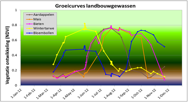
Figure 1. Growth curves of potatoes (brown), corn (orange), beets (pink), wheat (yellow) and flower bulbs (blue). Source: Roerink G. en Mucher S., “Nationaal Satelliet Dataportaal Ontsluiting en toepassingen”.
Figure 1 can be extended to perform classification to all the outputs required by the stakeholders (lilies, onions, carrots, etc.). Furthermore, these classifications can be made using a data driven approach, i.e. to use a model to classify crops based on their growth curves. Firstly, such a model needs to be trained on a labeled set of growth curves after which it can perform classification on new growth curves. The flow of such an approach would start with satellite images and end with classified crops, as can be seen in Figure 2.
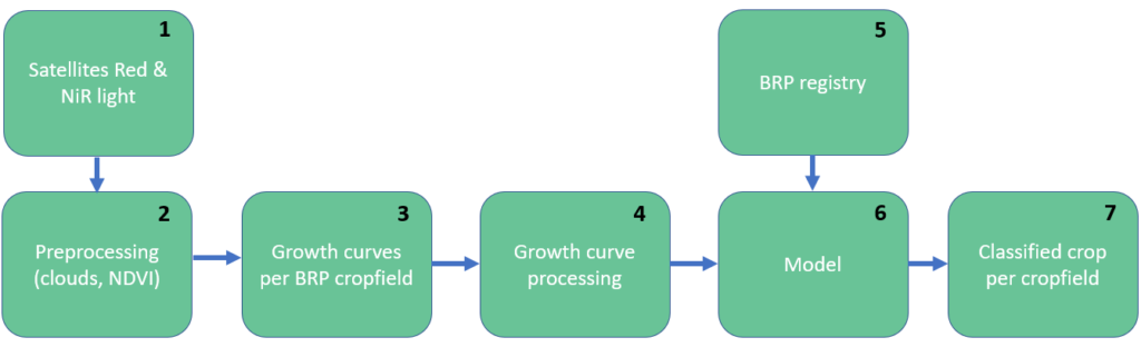
Figure 2. Steps to classify crops using a data driven approach. The raw data comes from Sentinel 2 multispectral images, this is shown in step 1. In step 2 atmospheric corrections are being performed and clouds are filtered from the images. Subsequently, the NDVI values are averaged over each BRP registry parcel in step 3. In step 4 temporal post processing steps such as interpolation and applying a moving average are being carried out on the images. Now the processed NDVI curves can be fed into a classifier, which is depicted in step 6. During training the BRP registered crops are used as ground truth, such that the model is trained to predict the correct crop at test time (shown in step 5 and 6 respectively)
In order to use supervised classification methods, ground-truth labels are required to train a model. This ground truth data is taken from the Basisregistratie Gewaspercelen (BRP). The BRP is an open data set that contains parcels with labeled crops for each agricultural field in the Netherlands. Now that we have our ground truth labels, we still need to generate our input. To not reinvent the wheel, we partnered up with The Wageningen University & Research (WUR), who supply us with aggregated NDVI values per BRP parcel, from processed Sentinel-2 satellite images. This means that the missing links in Figure 2 are steps 4, 6 and 7. Time to get our hands dirty.
Step 4 concerns the processing of growth curves. The upper graph in Figure 3 shows the growth curves as provided by the WUR. Firstly we filter the zeroes (clouds) and interpolate to acquire evenly spread values, this can be seen in the middle plot. Lastly we apply a moving average to smooth out the curve, this results in the lower plot which is the input for our model.
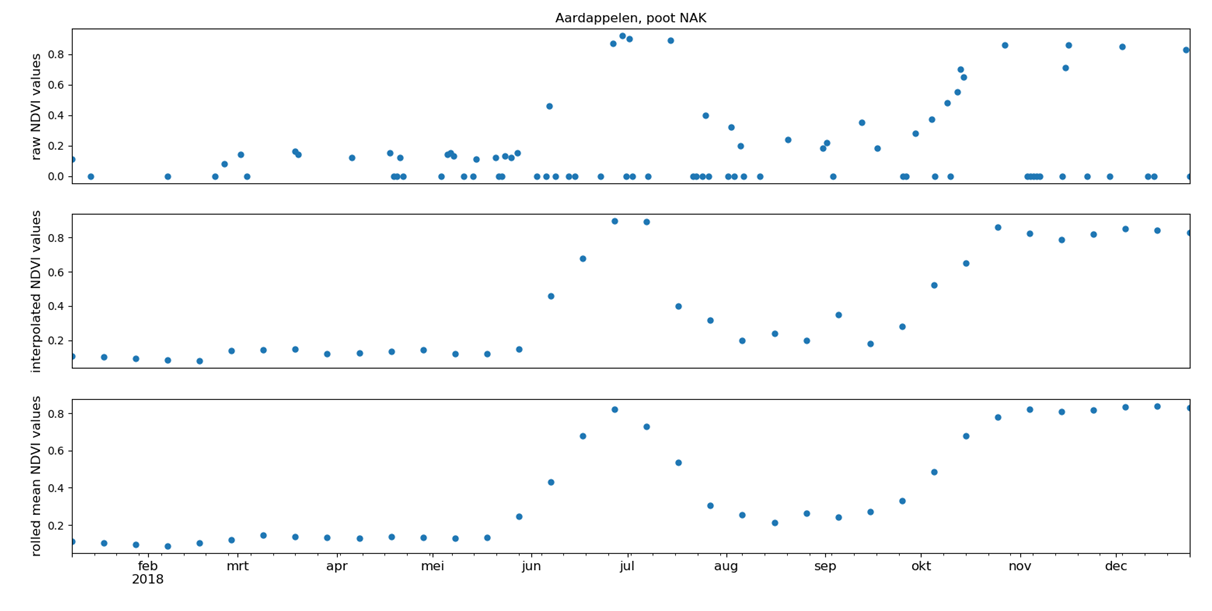
Figure 3. Processing a potato growth curve: Raw data is filtered and interpolated before a moving average is applied.
Before jumping to the model, we performed data exploration on the processed growth curves to see whether a model would indeed be capable of classification as suggested by Figure 1. Therefore, we looked at the variation in growth curves between different crops. This determines the success of the model: the more variance between growth curves, the easier it is to perform classification. Figure 4 and 5 show boxplots of growth curves associated with potatoes and with wheat. There is quite some variation in the growth curves between these two crops. However, we also found partial overlapping growth curves, such as potatoes and corn, which might therefore proof challenging to distinguish.
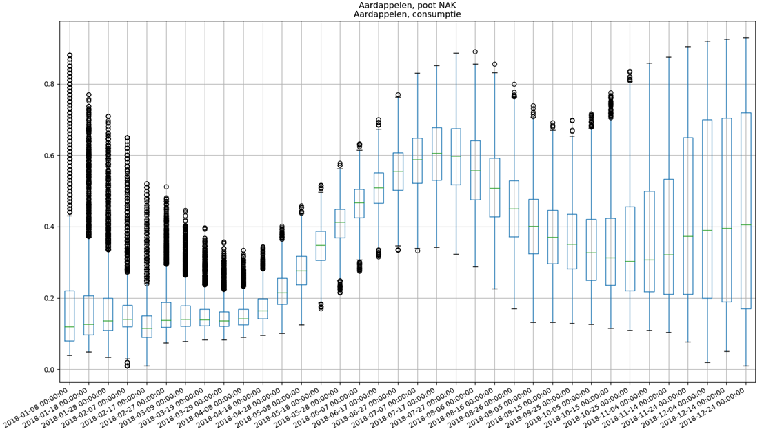
Figure 4. Boxplot of approximately 2500 processed potato growth curves.
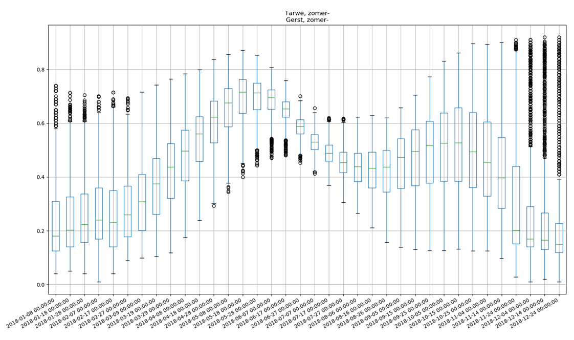
Figure 5. Boxplot of approximately 2000 processed wheat growth curves.
Looking at the variation between the growth curves, it appears that a model can be trained to classify the majority of crops based on their growth curves. However, such a model might have difficulty classifying between crops with similar growth curves such as corn and potatoes. Let’s find out by training a model!
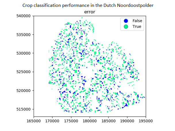
Figure 6. Performance (68% accurate) of model trained on growth curves from January until June. This plot shows the Noordoostpolder in the rijksdriehoekstelsel coordinate frame.
Figure 6 and 7 show the performance of two models on a validation test, with performances of 68% and 87%. These figures show the classification of all the crops grown on leased lands in the Dutch Noordoostpolder and the accuracy of the classification. The difference between the models is the duration on which they are trained. Figure 6 is trained to classify growth curves from January until June, Figure 7 is trained until August. The resulting difference in performance is logical because the crops undergo their biggest transformation during the summer months. Therefore, the incorporation of these months greatly increases the variation of growth curves and as a result, the performance of the model.
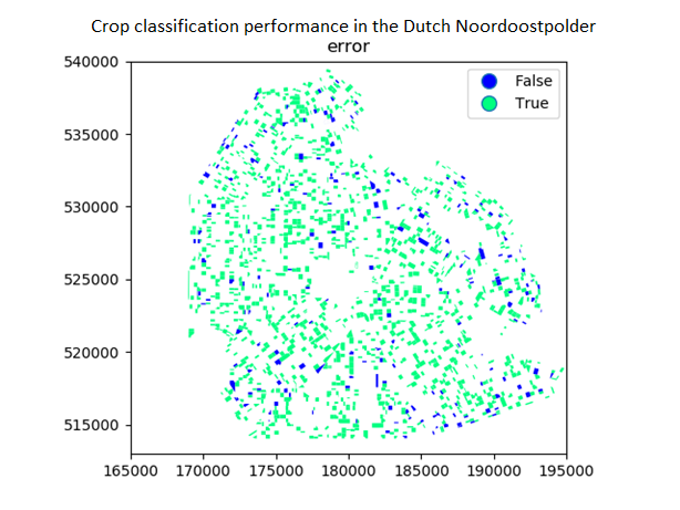
Figure 7. Performance (87% accurate) of model trained on growth curves from January until August. This plot shows the noordoostpolder in the rijksdriehoekstelsel coordinate frame.
This insight in the tradeoff between performance and time of classification was essential for a consumer fit product: The end user needs to act on the results of the classification. However, by the end of september all proof of the correctness of the classification will have vanished because farmers will have started ploughing their lands. Therefore, we agreed on a number of classifying moments with increasing performance.
Furthermore, we got the essential insight of the incompleteness of our solution: our approach classifies crops in fixed polygons, namely the shapes registered in the BRP. However, a farmer could crop his lands in different shapes than registered. In such a situation our model would be detached from reality and offer unusable insights. To overcome this problem we are going to classify on pixels instead of fixed polygons. From this pixel classification the actual shapes of the lands can be determined, namely clusters of similar pixels.
At the end of the meeting we discussed the use of closed data sources (which we are going to need to hold our results against rotation rules) and the GDPR, the integration of our solution into their IT department and the way in which the end users want to use the visualisation tool.
Our path forward is clear: classify pixels. Currently we are discussing the possibility of using growth curves per pixel provided by the WUR. In addition, we are looking into using Sentinel-1 RADAR images to expand the input of the model. This should reduce the confusion between crops with similar growth curves, such as corn and potatoes. We will keep you up to date!
![On satellites, growth curves and the birth of the Crop Detector [3]](https://geronimo.ai/wp-content/uploads/2019/11/faulty_parcels_1338x769-min-768x441.png)