Welcome to the second blog about Naive Bayes! Part II will build upon its ancestor, so many techniques from Part I will be left unexplained and are directly used in this blog. In case you missed the first blog, we recommend you read that first. Last time we presented the Naive Bayes classifier for text classification. The goal of the investigation presented in this blog is twofold. First of all, we are interested in reaching the highest possible accuracy when using the Naive Bayes classifier. Second, we will explore the trade-off in performance vs computational power by considering the number of features that is needed to reach the performance. 

In the previous blog we varied feature representation, stop word removal, tokenizer type and lemmatization to see their impact on the performance. In this blog we will extend this analysis by varying the N-gram range, the document frequency and the tuning parameter. No idea what these terms mean? No worries, we will explain them along the way!

N-gram range comparison

Sk-learn offers the possibility to build N-grams from the words. An N-gram is a newly created feature by combining N consecutive words with the purpose to extract more value from the data. For example, the word “movie” does not relate strongly to either the class positive or negative whereas “horrible movie” relates strongly to a negative review. The N-gram range says something about the type of N-grams that are considered and is given as tuple. For example; the N-grams in range (1,3) of “this movies sucks” are “this”, “this movie”, “this movie sucks”, “movie”, “movie sucks” and “sucks”. The N-gram in range (3, 3) is given as “this movie sucks”, which is the only 3-gram that can be extracted from this short example. 

We will perform experiments that consider all 6 combinations from n_range = (1,1) to n_range = (3, 3). Furthermore, df_min is kept at 5, meaning that we only consider words that occur in 5 or more documents. The bag of words (BoW) and term frequency-inverse document frequency (TF-IDF) representations are compared, as well as stop word removal vs. no stop word removal. Furthermore, for all experiments presented in this blog we cross-validate over the data and present the average of all metrics. The results are presented in Figure 1, split on stop word removal and no stop word removal. The experiments are plotted with their average test accuracy vs. their average number of features. The corresponding n-gram range is plotted in the figure.

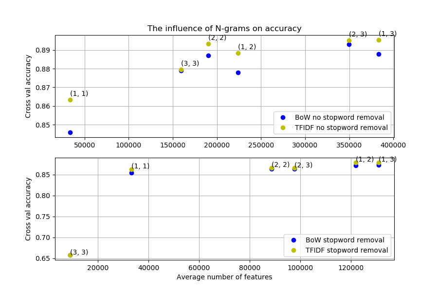
When analysing the experiments where no stop words are removed, we can observe the following:

1. Adding N-grams as features is beneficial for the accuracy.
2. TF-IDF outperforms BoW.
3. A sentence with Q unique words result in Q-(N-1) features, where N is the N-gram considered. So the number of features F for a corpus with unique words when considering 1,2 and 3-grams would result in F_{(1, 1)} > F_{(2, 2)} > F_{(3, 3)}. Differences in this order is caused by non-unique features and features with a document frequency lower than the lower threshold document frequency df_min.
4. Somehow, the N-gram range (2, 2) is outperforming (1, 2) for both BoW and TF-IDF. This is very odd, as (1, 2) contains both single words and 2-grams as features.

Analysing the experiments where stop words are removed, we observe the following:

1. A higher average number of features generally results in a higher performance and TF-IDF still outperforms BoW.
2. If we compare the average number of features for the experiments where the stop words are not removed, we can see that they are way lower. Removing stop words results in a set of scarce features which are filtered out by applying the lower threshold on the document frequency. Think about it, discarding stop words basically removes the most common links between sentence, leaving them as a bunch of non-connected unique variation of words.
3. The experiment with range (1, 2) reaches the highest accuracy. The experiment with range (1, 3) does not perform better despite it having more features. The set of 3 N-grams does not increase the accuracy, because by removing the stop words first and then combining the three consecutive words the contextual information of the words is destroyed.

Generally speaking, N-grams improve the accuracy! So that is nice. Let’s see how the accuracy behaves after thresholding the document frequency. So far we have used df_min = 5 as ball-park estimate to alleviate the calculations. In the next paragraph we will discover whether this is a decent parameter choice.

Influence of the document frequency

By varying the maximum and minimum document (df_max and df_min) frequency logarithmically, we will investigate its impact on the performance of Naive Bayes. The document frequency of a term is defined as the number of documents it has occurred in when vocabulary was built. Thresholding on the maximum and minimum document frequency thus means:

With df_max = m terms that occur in more than m documents are ignored.
With df_min = n terms that occur in less than n documents are ignored.

Minimum document frequency
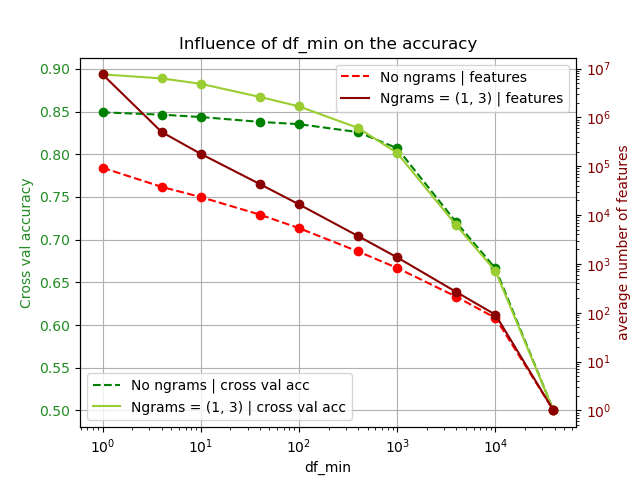
The minimum doc frequency is varied as df_min = [1, 4, 10, 40 , …, 10000, 39000]. 40000 was not possible to be used as df_min, since that resulted in a run where all features are ignored. Furthermore, N-grams are considered and please note that stopwords are not removed and only BoW is considered. The average cross val accuracy is plotted against the corresponding average number of features in Figure 2.

 We can observe the following:

1. When comparing the experiments with N-grams vs. no N-grams, we can see that the accuracy decreases faster as df_min increases for the experiments where N-grams were applied. The N-gram features generate a lot of new infrequently appearing features. These scarce features are filtered out more as the minimum document frequency increases, resulting in a stronger decrease in number of features and therefore resulting in a stronger decrease in performance
2. When we don’t apply N-grams and consider the range df_min = [1, 400], we observe that there is little impact on the test accuracy, while the number of features decreases significantly. From the perspective of features vs. accuracy, this is an interesting observation.
3. When we focus on the range df_min = [1000, 39000], there is little difference in performance between the experiments with N-grams and without N-grams. There is however, a difference in number of features.

The difference in number of features at df_min = 5 is significant. However, we can see that the corresponding accuracy loss is minimal. Therefore, the estimate of df_min = 5 was reasonable.

Maximum document frequency
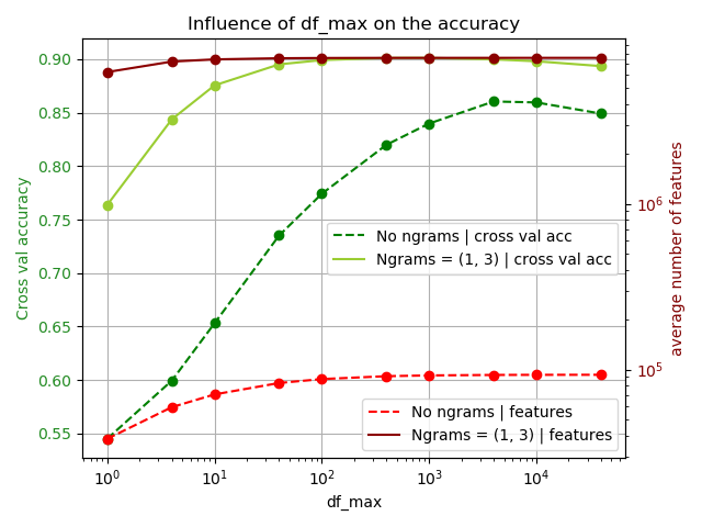
The maximum document frequency is varied as df_max = [1, 4, 10, 40 , …, 10000, 40000] Once again, stopwords are not removed and only BoW is considered. The results are presented in Figure 3.

We can observe the following: 

1. The difference in performance between N-grams and no N-grams is significant throughout the entire range of df_max.
2. There is a significant difference in average number of features between N-grams and no N-grams throughout the entire range of df_max.
3. The accuracy when df_max < 10 is surprisingly high, especially when N-grams are considered. For example, the accuracy for df_max = 1 is ~76%. This accuracy is reached if we only consider features that occur once. The number of features for this experiment is roughly 6 million.
4. Words like “movie” occur in basically every positive and negative review. Filtering out features with such high document frequency paves way for features that point strongly towards a sentiment.  As we increase the df_max, we see that these words are no longer filtered out and observe a decrease in performance after df_max = 10,000.

Influence of feature selection

Sk-learn offers many feature selection methods, from which we’ll explore two; the chi-square test (sklearn.feature_selection.chi2) and the ANOVA test (sklearn.feature_selection.f_classif). To measure the impact of the feature selection methods, we’ll compare them with the k most frequent features. The experiments are run without removing the stop words, df_min = 5 and N-gram range = (1, 3). The number of features k is varied as k = [1, 10, … , 100.000, all]

When we look at Figure 4, we can make a few observations:

1. Generally, as the number of features increase, the accuracy increases. However, the highest accuracy is reached at k = 10^5.
2. It is beneficial to use a feature selector throughout the whole range of number of features.
3. Combining a feature selector with TF-IDF is beneficial for the performance. 

To get a feel for features that have impact, the features selected by ANOVA for the experiment with k = 100 are presented below. The corresponding test accuracy of this single run is 0.8071. The features are given below:

[‘acting’ ‘also’ ‘always’ ‘amazing’ ‘an excellent’ ‘and’ ‘annoying’ ‘any’ ‘as’ ‘as the’ ‘at all’ ‘at least’ ‘avoid’ ‘awful’ ‘bad’ ‘bad acting’ ‘bad it’ ‘badly’ ‘beautiful’ ‘beautifully’ ‘best”boring’ ‘both’ ‘brilliant’ ‘cheap’ ‘could’ ‘crap’ ‘don’ ‘don waste’ ‘dull’ ‘even’ ‘excellent’ ‘fantastic’ ‘favorite’ ‘great’ ‘highly’ ‘his’ ‘horrible’ ‘if’ ‘instead’ ‘is great’ ‘is one of’ ‘it just’ ‘just’ ‘lame’ ‘laughable’ ‘least’ ‘life’ ‘love’ ‘loved’ ‘mess’ ‘minutes’ ‘money’ ‘movie’ ‘must see’ ‘no’ ‘not even’ ‘nothing’ ‘of the best’ ‘of the worst’ ‘oh’ ‘one of’ ‘pathetic’ ‘perfect’ ‘plot’ ‘pointless’ ‘poor’ ‘poorly’ ‘ridiculous’ ‘script’ ‘so bad’ ‘stupid’ ‘superb’ ‘supposed’ ‘supposed to’ ‘supposed to be’ ’terrible’ ’the acting’ ’the best’ ’the only’ ’the worst’ ’the worst movie’ ’thing’ ’this’ ’today’ ‘unless’ ‘very’ ‘waste’ ‘waste of’ ‘waste of time’ ‘waste your’ ‘waste your time’ ‘wasted’ ‘well’ ‘why’ ‘wonderful’ ‘worse’ ‘worst’ ‘worst movie’ ‘your time’]

Here we do see some shortcomings of the feature selector. We see a lot of repetitive features (“the worst movie”, “worst movie”). Here we can ask ourselves whether there is a way to prevent the feature selector from selecting almost identical features.

We saw that the feature selector is mainly beneficial in the situation where computation power is very (very) expensive. It is a great method for selecting a small set of features to reach a decent accuracy. Unfortunately, the overall increase in accuracy by using a feature selector is minimal. Let’s see if the alpha parameter is adding any accuracy.

Influence of the alpha parameter

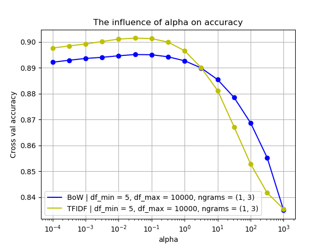
Generally, an alpha parameter is added to prevent that an unseen word in the test set cancels out all chances by multiplying it with 0. The influence of alpha on the test accuracy for both BoW and TF-IDF is presented in Figure 5. In the experiments we used the settings that gave promising results. The settings used are df_min = 5, df_max = 10000, ngram_range = (1, 3). 

Funny enough, for both representations the peak is not at 1 but at 0.031, while 1 is the default setting. Furthermore, we can see that the performance of TF-IDF drops below BoW from and higher.

Conclusion

By using a threshold on the df_max and df_min, applying N-grams, TF-IDF and by varying we reach an accuracy of 0.9014 which is impressive if you consider the nature of the classifier we are using.

Now let’s put this number into context. Using a Logistic Regression classifier with the exact same pre-processing steps (thresholding document frequency, N-grams and TF-IDF) results in an average score of 0.9077. This kernel uses TF-IDF, ngram_range = (1, 2) and selects the 20.000 best features using ANOVA. The classifier used, is a fully connected sigmoid network with one hidden layer with 64 neurons each and 20.000 inputs. The classifier reaches a whopping 0.9311 accuracy on a 0.8/0.2 train/test split. This kernel represents reviews as integers, where every integer corresponds with a word from the corpus. As classifier a neural network with 2 convolutional layers and 2 bi-directional LSTM layers is used. It reaches 0.88 accuracy on a 0.8/0.2 train/test split.

We hope this blog gave you an insight into the impact of the parameters on the accuracy. In part III of the blog we will investigate the performance of the Naive Bayes classifier on unbalanced data sets.